k1lib.viz module

This module is for nice visualization tools. This is exposed automatically with:

from k1lib.imports import *
viz.mask # exposed

k1lib.viz.daisyUI()

Grabs a nice subset of DaisyUI, just enough for a dynamic site that looks good enough

class k1lib.viz.SliceablePlot(plotF: Callable[[slice], None], slices: slice | List[slice] = slice(None, None, None), plotDecorators: List[_PlotDecorator] = [], docs='')

This is a plot that is “sliceable”, meaning you can focus into a particular region of the plot quickly. A minimal example looks something like this:

import numpy as np, matplotlib.pyplot as plt, k1lib
x = np.linspace(-2, 2, 100)

def normalF():
    plt.plot(x, x**2)

@k1lib.viz.SliceablePlot.decorate
def plotF(_slice):
    plt.plot(x[_slice], (x**2)[_slice])

plotF()[70:] # plots x^2 equation with x in [0.8, 2]

So, normalF plots the equation \(x^2\) with x going from -2 to 2. You can convert this into a SliceablePlot by adding a term of type slice to the args, and decorate with decorate(). Now, every time you slice the SliceablePlot with a specific range, plotF will receive it.

How intuitive everything is depends on how you slice your data. [70:] results in x in [0.8, 2] is rather unintuitive. You can change it into something like this:

@k1lib.viz.SliceablePlot.decorate
def niceF(_slice):
    n = 100; r = k1lib.Range(-2, 2)
    x = np.linspace(*r, n)
    _slice = r.toRange(k1lib.Range(n), r.bound(_slice)).slice_
    plt.plot(x[_slice], (x**2)[_slice])
# this works without a decorator too btw: k1lib.viz.SliceablePlot(niceF)

niceF()[0.3:0.7] # plots x^2 equation with x in [0.3, 0.7]
niceF()[0.3:] # plots x^2 equation with x in [0.3, 2]

The idea is to just take the input slice, put some bounds on its parts, then convert that slice from [-2, 2] to [0, 100]. Check out k1lib.Range if it’s not obvious how this works.

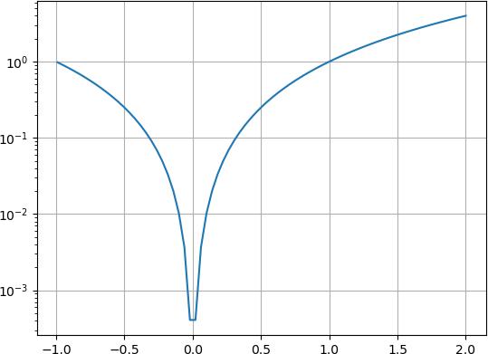
A really cool feature of SliceablePlot looks like this:

niceF().legend(["A"])[-1:].grid(True).yscale("log")

This will plot \(x^2\) with range in [-1, 2] with a nice grid, and with y axis’s scale set to log. Essentially, undefined method calls on a SliceablePlot will translate into plt calls. So the above is roughly equivalent to this:

x = np.linspace(-2, 2, 100)
plt.plot(x, x**2)
plt.legend(["A"])
plt.grid(True)
plt.yscale("log")

This works even if you have multiple axes inside your figure. It’s wonderful, isn’t it?

static decorate(f)

Decorates a plotting function so that it becomes a SliceablePlot.

k1lib.viz.plotSegments(x: List[float], y: List[float], states: List[int], colors: List[str] = None)

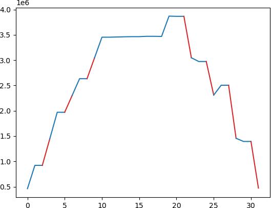
Plots a line graph, with multiple segments with different colors.

Idea is, you have a normal line graph, but you want to color parts of the graph red, other parts blue. Then, you can pass a “state” array, with the same length as your data, filled with ints, like this:

y = np.array([ 460800,  921600,  921600, 1445888, 1970176, 1970176, 2301952,
       2633728, 2633728, 3043328, 3452928, 3452928, 3457024, 3461120,
       3463680, 3463680, 3470336, 3470336, 3467776, 3869184, 3865088,
       3865088, 3046400, 2972672, 2972672, 2309632, 2504192, 2504192,
       1456128, 1393664, 1393664,  472576])
s = np.array([1, 0, 0, 1, 0, 0, 1, 0, 0, 1, 0, 0, 0, 0, 0, 0, 0, 0, 0, 0, 0, 0,
       1, 0, 0, 1, 0, 0, 1, 0, 0, 1])
plotSegments(None, y, s, colors=["tab:blue", "tab:red"])

Parameters:

• x – (nullable) list of x coordinate at each point

• y – list of y coordinates at each point

• states – list of color at each point

• colors – string colors (matplotlib color strings) to display for each states

class k1lib.viz.Carousel(searchMode: int = 0)

__init__(searchMode: int = 0)

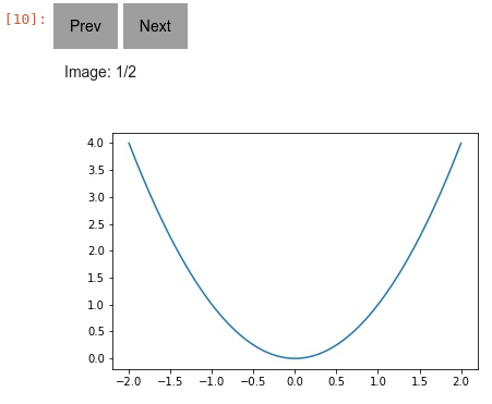
Creates a new Carousel that can flip through a list of images/html. Will even work even when you export the notebook as html. Example:

x = np.linspace(-2, 2); plt.plot(x, x ** 2); im1 = plt.gcf() | toImg()
x = np.linspace(-1, 3); plt.plot(x, x ** 2); im2 - plt.gcf() | toImg()
im3 = "<h1>abc</h1><div>Some content</div>" # can add html
[im1, im2, im3] | viz.Carousel() # displays in notebook cell

There’s also a builtin search functionality that works like this:

[
    "<h1>abc</h1><div>Some content 1</div>",
    "<h1>def</h1><div>Some other content 2</div>",
    "<h1>ghi</h1><div>Another content 3</div>",
] | viz.Carousel(searchMode=1)

[
    ["<h1>abc</h1>", "<div>Some content 1</div>"],
    ["<h1>def</h1>", "<div>Some other content 2</div>"],
    ["<h1>ghi</h1>", "<div>Another content 3</div>"],
] | viz.Carousel(searchMode=2)

The first mode will search for some text inside the html content. The second mode will search inside the title only, that means it’s expecting to receive Iterator[title, html/img]

Parameters:

• imgs – List of initial images. Can add more images later on by using __ror__()

• searchMode – 0 for no search, accepts Iterator[html/img], 1 for search content, accepts Iterator[html/img], 2 for search title, accepts Iterator[title, html/img]

__ror__(it)

Return value|self.

class k1lib.viz.Toggle

__init__()

Button to toggle whether the content is displayed or not. Useful if the html content is very big in size. Example:

x = np.linspace(-2, 2); plt.plot(x, x ** 2)
plt.gcf() | toImg() | toHtml() | viz.Toggle()

This will plot a graph, then create a button where you can toggle the image’s visibility

__ror__(it)

Return value|self.

class k1lib.viz.ToggleImage

This function is sort of legacy. It’s just img | toHtml() | viz.Toggle() really

class k1lib.viz.Scroll(height=300)

__init__(height=300)

Creates a new preview html component. If content is too long, then it will only show the first 500px, then have a button to expand and view the rest. Example:

x = np.linspace(-2, 2); plt.plot(x, x ** 2)
plt.gcf() | toImg() | toHtml() | viz.Scroll()

This will plot a preview of a graph :param height: height of the parent container

__ror__(it)

Return value|self.

k1lib.viz.confusionMatrix(matrix: Tensor, categories: List[str] = None, **kwargs)

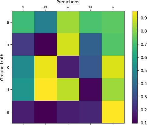
Plots a confusion matrix. Example:

k1lib.viz.confusionMatrix(torch.rand(5, 5), ["a", "b", "c", "d", "e"])

Parameters:

• matrix – 2d matrix of shape (n, n)

• categories – list of string categories

• kwargs – keyword args passed into plt.figure()

k1lib.viz.FAnim(fig, f, frames, *args, **kwargs)

Matplotlib function animation, 60fps. Example:

# line below so that the animation is displayed in the notebook. Included in :mod:`k1lib.imports` already, so you don't really have to do this!
plt.rcParams["animation.html"] = "jshtml"
x = np.linspace(-2, 2); y = x**2
fig, ax = plt.subplots()
plt.close() # close cause it'll display 1 animation, 1 static if we don't do this
def f(frame):
    ax.clear()
    ax.set_ylim(0, 4); ax.set_xlim(-2, 2)
    ax.plot(x[:frame], y[:frame])
k1lib.FAnim(fig, f, len(x)) # plays animation in cell

Parameters:

• fig – figure object from plt.figure(…) command

• f – function that accepts 1 frame from frames.

• frames – number of frames, or iterator, to pass into function

k1lib.viz.mask(img: Tensor, act: Tensor) → Tensor

Shows which part of the image the network is focusing on.

Parameters:

• img – the image, expected to have dimension of (3, h, w)

• act – the activation, expected to have dimension of (x, y), and with elements from 0 to 1.

class k1lib.viz.PDF(pdf: str = None, size=(700, 500))

__init__(pdf: str = None, size=(700, 500))

Displays pdf in the notebook. Example:

viz.PDF("a.pdf")
"a.pdf" | viz.PDF()

viz.PDF("a.pdf", (700, 500))
"a.pdf" | viz.PDF(size=(700, 500))

If you’re exporting this notebook as html, then you have to make sure you place the generated html file in the correct directory so that it can reference those pdf files.

Parameters:

pdf – relative path to pdf file

__ror__(pdf)

Return value|self.

class k1lib.viz.Html

A string that will display rich html to a notebook. Example:

s = "Just a <b>regular</b> string"
h = viz.Html(s) # this is an instance of viz.Html, but it's also still a string, as viz.Html subclasses str!
h               # running this in a notebook cell will display out the html

class k1lib.viz.onload

__init__()

Returns html code that will run the captured clis when that html is loaded. Example:

3 | (toJsFunc() | (viz.onload() | aS("x+3"))) | op().interface()

This displays html that will execute “x+3”, then inject it into the main body. At first glance, this seems useless. A much simpler solution exists:

3 | (toJsFunc() | aS("x+3")) | op().interface()

This would pretty much do the exact same thing. But there’s a subtle difference. The jsFunc output of the first line (the one with onload()) is some complex html, and of the second line (without onload()) is just a single number. This is useful in cases where you don’t want to render something right away (as that can take time/space), but want to defer rendering till later. This is roughly what the first line generates this html:

<div id="content">(Loading...)</div>
<script>
    const data = 3;
    const customFunction = (x) => x+3;
    function onload() { document.querySelector("#content").innerHTML = customFunction(data); }
    onload();
</script>

While the second line generates this html:

6

These html is returned by the blocks (viz.onload() | aS("x+3")) and aS("x+3") in JS, respectively.

The value of this is that your custom function might do something that generates a whole bunch of html (like fetching an image somewhere, then return the base64-encoded image tag). If you were to do it the normal way, then you would execute your function, return the giant html to display. Meanwhile, if you use this cli, then when you’re moving html around, it’s relatively lightweight, and only when that html is embedded into a page will your custom function captured by onload execute, and display outwards.

Honestly this feels like another implementation of toJsFunc

__ror__(it: str)

Return value|self.

class k1lib.viz.Clipboard(msg='Copy to clipboard')

__init__(msg='Copy to clipboard')

Returns some nice Html of a button that will copy to the clipboard when the user clicks on it. Example:

"some data" | viz.Clipboard() # returns html string

Parameters:

msg – message on the button

__ror__(it)

Return value|self.

class k1lib.viz.Download(fn: str = 'untitled', msg: str = 'Download file')

__init__(fn: str = 'untitled', msg: str = 'Download file')

Returns some nice Html of a button that will download whatever’s piped into this into a file. Example:

"some data" | viz.Download("some_text_file.txt") # returns html string that downloads the file

Parameters:

• fn – desired file name

• msg – message on the button

__ror__(it)

Return value|self.

class k1lib.viz.qrScanner(fName=None, facing='environment')

Returns some nice Html displaying a live video feed that calls a function when a QR code is identified. Example:

ht = viz.qrScanner("qrIdentified")
viz.Html(ht + "<script>function qrIdentified(data) { console.log("qr: ", data); }</script>")

After executing that in a cell, it should display a live video feed

Parameters:

• fName – js function name to be triggered

• facing – ‘environment’ or ‘user’, determines the camera location

class k1lib.viz.Popup(elem: str, popup: str)

Makes an popup appear at the bottom right of an element after clicking on it. Example:

a = viz.Popup("<button>abc</button>", "<div>popup content</div>")
b = f"{a}<pre>some\nother\ncontent</pre>" | toHtml()

class k1lib.viz.Table(headers: list[str] = None, onclickFName: str = None, ondeleteFName: str = None, oneditFName: str = None, onclickHeaderFName: str = None, colOpts: list[list[str]] = None, sortF: str = None, selectable=False, selectCallback: str = None, height=None, objName: str = None, colsToHide: list[int] = None, perPage: int = None, numRows=None)

__init__(headers: list[str] = None, onclickFName: str = None, ondeleteFName: str = None, oneditFName: str = None, onclickHeaderFName: str = None, colOpts: list[list[str]] = None, sortF: str = None, selectable=False, selectCallback: str = None, height=None, objName: str = None, colsToHide: list[int] = None, perPage: int = None, numRows=None)

Returns some nice Html displaying a table. Example:

res = enumerate("abcdef") | viz.Table(onclickFName="onclickF", ondeleteFName="deleteF")
f"""<script>
    function onclickF(row, i, e) {{ console.log("onclickF: ", row, i, e); }}
    function deleteF(row, i, e) {{ console.log("deleteF: ", row, i, e); }}
</script>
{res}""" | toHtml() # creates html string and displays it in the notebook cell

Normally, if you want to display a plain old table, you can do sometable | display(), which is the same as sometable | head() | pretty() | stdout(), but that only gives you a static table. This class will still show the table, but you can specify an “onclickFName” which the system will call whenever the user clicks on a particular row. If “ondeleteFName” is specified, then a column full of delete buttons will be injected as the first column, and if the user clicks on it will execute the function you specified. The example above should be intuitive enough.

If oneditFName is specified, then it allows editing a row at a time. After the user has typed in everything, that function will be called, and if successful, will update the table right away.

There’re these available options for each column (“colOpts”):

• [“pad”, 10]: padding on all 4 sides, defaulted to 10 if not specified

• “json”: if specified, will assume the row element to be a json and make it look nice

• [“jsonWidth”, 400]: max width of json fields

• [“jsonHeight”, 300]: max height of json fields

• “clipboard”: if specified, will copy the contents of the cell to clipboard when user clicks on it

Say you have 3 columns, and you want:

• Column 1: json with max width of 500px, copies its contents to clipboard onclick

• Column 2: nothing special

• Column 3: copies its contents to clipboard onclick

Then “colOpts” should be [[“json”, [“jsonWidth”, 500], “clipboard”], [], [“clipboard”]]

With tables that have complex features, there’s also a hidden “{pre}_obj” JS object that has a bunch of useful functions, as well as callbacks that allows you to do interactive things:

ui1 = enumerate("abcdef") | viz.Table(objName="something")
f"""
    {ui1}
    <script>
        setTimeout(() => something.update([[1, 2], [3, 4], [5, 6]]), 1000); // updates the table's contents after 1 second
        setTimeout(() => console.log(something.data), 3000); // prints the table's data after 3 seconds
    </script>
""" | toHtml()

Pagination {pre}_obj values:

• async page_select(pageNum:int): selects a specific page, 0-indexed

• async page_next(): goes to next page

• async page_prev(): goes to previous page

• async page_onselect(pageNum): function that should return list[list[str|int]] for the specific page it’s on. The returned result will be used to render the table. Don’t have to override this by default, it will just slice up the incoming data to return the correct page

Parameters:

• headers – a list of column names

• onclickFName – global function that will be called whenever the user clicks on a specific item

• ondeleteFName – global function that will be called whenever the user wants to delete a specific row

• oneditFName – global function that will be called whenever the user finishes editing a specific row

• onclickHeaderFName – global function that will be called whenever the user clicks on a specific header

• colOpts – column options

• sortF – takes in [table (list[list[str | number]]), col (int)] and returns the sorted table. Can put True in for the default sorter

• selectable – if True, make the row bold when user clicks on it, else don’t do that

• selectCallback – function name to inject into global namespace so as to trigger

• height – if specified, limits the table height to this many pixels, and add a vertical scrolling bar

• objName – name of the JS object that contains functions to interact with the table

• colsToHide – list of column indexes to hide internal selection. Does not cascade to onclickFName

• perPage – if specified, splits the incoming data into multiple pages, and allow users to navigate around those pages

• numRows – in pagination mode, this variable will be used to display the initial total number of pages. Purely aestheetic, no function

__ror__(it) → Html

Return value|self.