Monkey patched classes

These are functionalities added to other libraries, or “monkey-patched” them. How is this possible? Check out k1lib.patch().

k1lib._monkey.dummy()

Does nothing. Only here so that you can read source code of this file and see what’s up.

Python builtins

str.splitCamel()

Splits a string up based on camel case. Example:

# returns ['IHave', 'No', 'Idea', 'What', 'To', 'Put', 'Here']
"IHaveNoIdeaWhatToPutHere".splitCamel()

Class torch.nn.Module

Module.getParamsVector() → List[Tensor]

For each parameter, returns a normal distributed random tensor with the same standard deviation as the original parameter

Module.importParams(params: List[Parameter])

Given a list of torch.nn.parameter.Parameter/torch.Tensor, update the current torch.nn.Module’s parameters with it’

Module.exportParams() → List[Tensor]

Gets the list of torch.Tensor data

Module.paramsContext()

A nice context manager for importParams() and exportParams(). Returns the old parameters on enter context. Example:

m = nn.Linear(2, 3)
with m.paramsContext() as oldParam:
    pass # go wild, train, mutate `m` however much you like
# m automatically snaps back to the old param

Small reminder that this is not foolproof, as there are some Module that stores extra information not accessible from the model itself, like BatchNorm2d.

Module.deviceContext(buffers: bool = True) → ContextManager

Preserves the device of whatever operation is inside this. Example:

import torch.nn as nn
m = nn.Linear(3, 4)
with m.deviceContext():
    m.cuda() # moves whole model to cuda
# automatically moves model to cpu

This is capable of preserving buffers’ devices too. But it might be unstable. Parameter are often updated inline, and they keep their old identity, which makes it easy to keep track of which device the parameters are on. However, buffers are rarely updated inline, so their identities change all the time. To deal with this, this does something like this:

devices = [buf.device for buf in self.buffers()]
yield # entering context manager
for buffer, device in zip(self.buffers(), devices):
    buffer.data = buffer.data.to(device=device)

This means that while inside the context, if you add a buffer anywhere to the network, buffer-device alignment will be shifted and wrong. So, register all your buffers (aka Tensors attached to Module) outside this context to avoid headaches, or set buffers option to False.

If you don’t know what I’m talking about, don’t worry and just leave as default.

Parameters

buffers – whether to preserve device of buffers (regular Tensors attached to Module) or not.

Module.gradContext()

Preserves the requires_grad attribute. Example:

m = nn.Linear(2, 3)
with m.gradContext():
    m.weight.requires_grad = False
# returns True
m.weight.requires_grad

It’s worth mentioning that this does not work with buffers (Tensors attached to torch.nn.Module), as buffers are not meant to track gradients!

Module.__ror__(x)

Allows piping input to torch.nn.Module, to match same style as the module k1lib.cli. Example:

# returns torch.Size([5, 3])
torch.randn(5, 2) | nn.Linear(2, 3) | cli.shape()

Module.select(css: str = '*') → ModuleSelector

Creates a new ModuleSelector, in sync with a model. Example:

mS = selector.select(nn.Linear(3, 4), "#root:propA")

Or, you can do it the more direct way:

mS = nn.Linear(3, 4).select("#root:propA")

Parameters

• model – the torch.nn.Module object to select from

• css – the css selectors

Module.nParams

Get the number of parameters of this module. Example:

# returns 9, because 6 (2*3) for weight, and 3 for bias
nn.Linear(2, 3).nParams

Class torch.Tensor

Tensor.crissCross() → Tensor

Concats multiple 1d tensors, sorts it, and get evenly-spaced values. Also available as torch.crissCross() and crissCross(). Example:

a = torch.tensor([2, 2, 3, 6])
b = torch.tensor([4, 8, 10, 12, 18, 20, 30, 35])

# returns tensor([2, 3, 6, 10, 18, 30])
a.crissCross(b)

# returns tensor([ 2,  4,  8, 10, 18, 20, 30, 35])
a.crissCross(*([b]*10)) # 1 "a" and 10 "b"s

# returns tensor([ 2,  2,  3,  6, 18])
b.crissCross(*([a]*10)) # 1 "b" and 10 "a"s

Note how in the second case, the length is the same as tensor b, and the contents are pretty close to b. In the third case, it’s the opposite. Length is almost the same as tensor a, and the contents are also pretty close to a.

Tensor.histBounds(bins=100) → Tensor

Flattens and sorts the tensor, then get value of tensor at regular linspace intervals. Does not guarantee bounds’ uniqueness. Example:

# Tensor with lots of 2s and 5s
a = torch.Tensor([2]*5 + [3]*3 + [4] + [5]*4)
# returns torch.tensor([2., 3., 5.])
a.histBounds(3).unique()

The example result essentially shows 3 bins: \([2, 3)\), \([3, 5)\) and \([5, \infty)\). This might be useful in scaling pixels so that networks handle it nicely. Rough idea taken from fastai.medical.imaging.

Tensor.histScaled(bins=100, bounds=None) → Tensor

Scale tensor’s values so that the values are roughly spreaded out in range \([0, 1]\) to ease neural networks’ pain. Rough idea taken from fastai.medical.imaging. Example:

# normal-distributed values
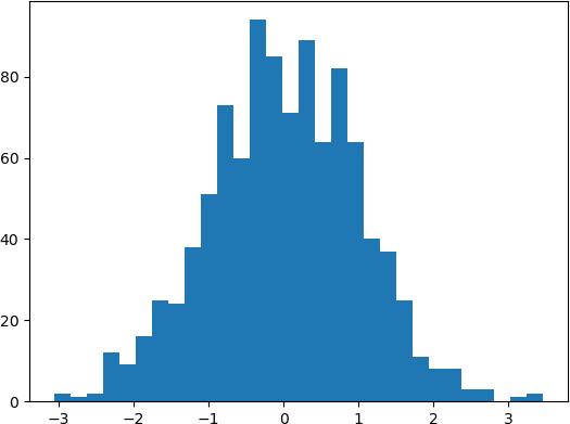
a = torch.randn(1000)
# plot #1 shows a normal distribution
plt.hist(a.numpy(), bins=30); plt.show()
# plot #2 shows almost-uniform distribution
plt.hist(a.histScaled().numpy()); plt.show()

Plot #1:

Plot #2:

Parameters

• bins – if bounds not specified, then will scale according to a hist with this many bins

• bounds – if specified, then bins is ignored and will scale according to this. Expected this to be a sorted tensor going from min(self) to max(self).

Tensor.positionalEncode(richFactor: float = 2) → Tensor

Position encode a tensor of shape \((L, F)\), where \(L\) is the sequence length, \(F\) is the encoded features. Will add the encodings directly to the input tensor and return it.

This is a bit different from the standard implementations that ppl use. This is exactly:

\[p = \frac{i}{F\cdot richFactor}\]

\[w = 1/10000^p\]

\[pe = sin(w * L)\]

With i from range [0, F), and p the “progress”. If richFactor is 1 (original algo), then p goes from 0% to 100% of the features. Example:

import matplotlib.pyplot as plt, torch, k1lib
plt.figure(dpi=150)
plt.imshow(torch.zeros(100, 10).positionalEncode().T)

Parameters

richFactor – the bigger, the richer the features are. A lot of times, I observe that the features that are meant to cover huge scales are pretty empty and don’t really contribute anything useful. So this is to bump up the usefulness of those features

Tensor.clearNan(value: float = 0.0) → Tensor

Sets all nan values to a specified value. Example:

a = torch.randn(3, 3) * float("nan")
a.clearNan() # now full of zeros

Tensor.hasNan() → bool

Returns whether this Tensor has any nan values at all.

Tensor.hasInfs()

Whether this Tensor has negative or positive infinities.

Module torch

torch.loglinspace(b, n=100, **kwargs)

Like torch.linspace(), but spread the values out in log space, instead of linear space. Different from torch.logspace()

torch.sameStorage(b)

Check whether 2 (numpy.ndarray or torch.Tensor) has the same storage or not. Example:

a = np.linspace(2, 3, 50)
# returns True
torch.sameStorage(a, a[:5])
# returns True
torch.sameStorage(a[:10], a[:5])
returns false
torch.sameStorage(a[:10], np.linspace(3, 4))

All examples above should work with PyTorch tensors as well.

Class graphviz.Digraph

Digraph.__call__(_from, *tos, **kwargs)

Convenience method to quickly construct graphs. Example:

g = k1lib.graph()
g("a", "b", "c")
g # displays arrows from "a" to "b" and "a" to "c"

Class graphviz.Graph

Graph.__call__(_from, *tos, **kwargs)

Convenience method to quickly construct graphs. Example:

g = k1lib.graph()
g("a", "b", "c")
g # displays arrows from "a" to "b" and "a" to "c"

Class mpl_toolkits.mplot3d.axes3d.Axes3D

Axes3D.march(heatMap, level: float = 0, facecolor=[0.45, 0.45, 0.75], edgecolor=None)

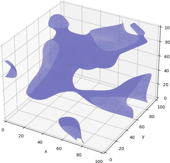
Use marching cubes to plot surface of a 3d heat map. Example:

plt.k3d(6).march(k1lib.perlin3d(), 0.17)

A more tangible example:

t = torch.zeros(100, 100, 100)
t[20:30,20:30,20:30] = 1
t[80:90,20:30,40:50] = 1
plt.k3d().march(t.numpy())

The function name is “march” because how it works internally is by using something called marching cubes.

Parameters

• heatMap – 3d numpy array

• level – array value to form the surface on

Axes3D.surface(z, **kwargs)

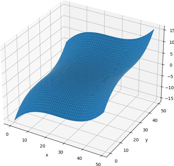
Plots 2d surface in 3d. Pretty much exactly the same as plot_surface(), but fields x and y are filled in automatically. Example:

x, y = np.meshgrid(np.linspace(-2, 2), np.linspace(-2, 2))
plt.k3d(6).surface(x**3 + y**3)

Parameters

• z – 2d numpy array for the heights

• kwargs – keyword arguments passed to plot_surface

Axes3D.plane(origin, v1, v2=None, s1: float = 1, s2: float = 1, **kwargs)

Plots a 3d plane.

Parameters

• origin – origin vector, shape (3,)

• v1 – 1st vector, shape (3,)

• v2 – optional 2nd vector, shape(3,). If specified, plots a plane created by 2 vectors. If not, plots a plane perpendicular to the 1st vector

• s1 – optional, how much to scale 1st vector by

• s2 – optional, how much to scale 2nd vector by

• kwargs – keyword arguments passed to plot_surface()

Axes3D.point(v, **kwargs)

Plots a 3d point.

Parameters

• v – point location, shape (3,)

• kwargs – keyword argument passed to scatter()

Axes3D.line(v1, v2, **kwargs)

Plots a 3d line.

Parameters

• v1 – 1st point location, shape (3,)

• v2 – 2nd point location, shape (3,)

• kwargs – keyword argument passed to plot()

Module matplotlib.pyplot

pyplot.k3d(labels=True, *args, **kwargs)

Convenience function to get an Axes3D.

Parameters

• labels – whether to include xyz labels or not

• size – figure size

pyplot.animate(azimStart=0, elevSpeed=0.9, elevStart=0, frames=20, close=True)

Animates the existing 3d axes. Example:

plt.k3d().scatter(*np.random.randn(3, 10))
plt.animate()

Parameters

• frames – how many frames to render? Frame rate is 30 fps

• close – whether to close the figure (to prevent the animation and static plot showing at the same time) or not

pyplot.getFig()

Grab figure of the current plot. Example:

plt.plot() | plt.getFig() | toImg()

Internally, this just calls plt.gcf() and that’s it, pretty simple. But I usually plot things as a part of the cli pipeline, and it’s very annoying that I can’t quite chain plt.gcf() operation, so I created this

This has an alias called plt.toFig()

Module ray

ray.progress(title: str = 'Progress')

Manages multiple progress bars distributedly. Example:

with ray.progress(5) as rp:
    def process(idx:int):
        for i in range(100):
            time.sleep(0.05) # do some processing
            rp.update.remote(idx, (i+1)/100) # update progress. Expect number between 0 and 1
    range(5) | applyCl(process) | deref() # execute function in multiple nodes

This will print out a progress bar that looks like this:

Progress: 100% | 100% | 100% | 100% | 100%

Parameters

• n – number of progresses to keep track of

• title – title of the progress to show

Module os

os.netstat()

Runs netstat command and splits it up into a nice table. Example:

os.netstat() # returns [["Proto", "Recv-Q", "Send-Q", "Local Address", ...], [...], ...]

os.killPort(force: bool = False, allowMulti: bool = False)

Kills the process that is listening on a particular port. Example:

os.killPort(8888) # kill jupyterlab process, if it's running on this port

Parameters

• force – if True, will send SIGKILL, else send SIGTERM

• allowMulti – if True, allows multiple processes listening on the same port, else throws an error when that happens